Anyone who has used a computer for more than just playing games will be aware of spreadsheets. A spreadsheet is a versatile computer program (package) that enables you to do a wide range of calculations dynamically, and create high quality graphs and charts. Microsoft Excel is the most widely used spreadsheet, and is available within the Microsoft Office suite of programs.
As you work through this introduction to Excel, it is a good idea to be at a computer so that you can try out various things as they are described. To get into Excel, simply double click on the Microsoft Excel icon if there is one on the computer desktop.
Alternatively, click on the Start button in the bottom left corner of the screen, move the cursor to Programs to open up the programs menu, and then click on Microsoft Excel. Your computer should display the basic Excel screen as shown below.
Also Read: 50 Important Questions Related To Computer Technology
You are now ready to use Excel.

The bulk of the screen is devoted to displaying a spreadsheet, which is one of many similar sheets that make up an Excel workbook. By default, the workbook is set up with 3 sheets (Sheet1, Sheet2 and Sheet3), but this can be extended by creating additional sheets as required.
In simple examples, you will often be able to organise your work on a single sheet, but for more complicated problems it may be more convenient to use several sheets. Different sheets are accessed by clicking on the appropriate Tab at the bottom of the screen. It is also possible to give the sheets more meaningful names, rather than the default names Sheet1, Sheet2, Sheet3 etc. Simply right click on the Tab to open up a menu allowing you to (among other things) Insert, Delete or Rename the worksheet.
- Across the top of the screen is a title bar that displays the name of the program followed by the name of the workbook (“Book1” is the default name, which will change when you save your data under some other, more meaningful, name).
- On the right of the title bar are the usual buttons to minimise, maximise and close a window.
- Below the title bar is the main menu bar that contains a series of pull-down menus, organised as with most applications, into related groups of tasks. Selecting from the menu bar either opens up a sub-menu, or causes Excel to execute some task.
- Below the menu bar are two rows of toolbars that contain buttons (also called icons) for easy access to the more frequently used tasks. They allow you to execute the task by simply clicking on the appropriate button, rather than opening up a series of menus.
- Most of these buttons, such as cut or paste, are standard across many applications and work in exactly the same way as in, for example, Microsoft Word. You can also access some of these more common tasks by right-clicking on any part of the spreadsheet.
Note, however, that the part of the spreadsheet where you right-click, for instance a cell or a row or column header, will show a slightly different set of tasks that are appropriate to that element of the spreadsheet.
Suggested Read: Know Some of the Most Important Computer Full Forms
An Excel Spreadsheet
A spreadsheet works by laying out your data in a rectangular grid of rows and columns, in the same way that you would do if you were using a sheet of paper. For example, suppose you have collected quarterly data on home and export sales in the years 2003 and 2004. A natural way of displaying the data would be as shown below:
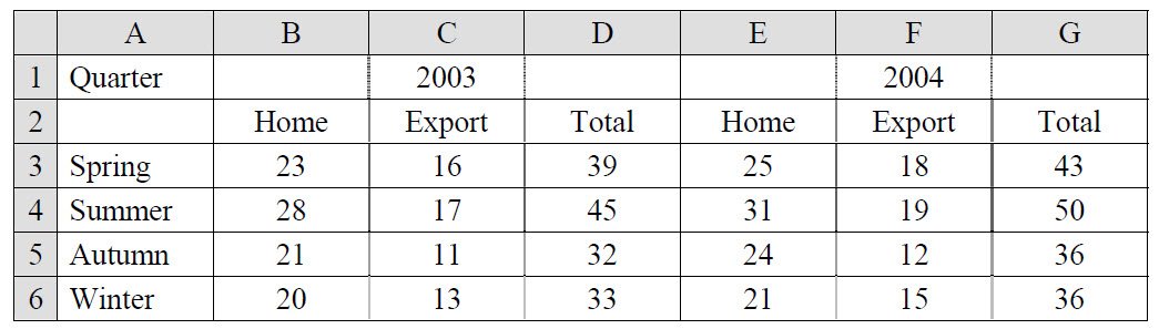
The data are laid out in 7 columns and 6 rows, including row and column headings. As you can see, in an Excel spreadsheet the rows are numbered from 1 upwards, and the columns are referred to by letters in alphabetical order.
After the 26th column, they are labelled AA, AB, AC, … then BA, BB, BC, … etc. When you have entered the data into Excel, what you see on the computer screen will look almost exactly like above screenshot, apart from some blank columns after G, and blank rows below 6.
Any cell in the spreadsheet is identified by its column and row position. For example, the top left cell containing the word “Quarter” is cell A1, and the home sales in autumn 2004 (the value 24) is in cell E5. We often need to refer to a range of cells, which is a rectangular block of consecutive rows and columns. For example, the 2003 data is contained in rows 3, 4, 5 and 6 of columns B, C and D.
In Excel, any range such as this is specified by the top left corner cell and the bottom right corner cell, separated by a colon. The 2003 data are therefore in the range B3:D6. Similarly, the 2004 export sales are in the range F3:F6, and all the sales data for 2004 are in the range E3:G6.
Entering and Adding Data
The cells of a spreadsheet can contain either numbers, as in cell B3, or characters (letters and other symbols), as in cell A1. To enter data into the spreadsheet, click on the appropriate cell and type in the required contents and then press Enter.
Immediately above the column headings of the spreadsheet, there is a Formula bar that shows the active cell address, and the contents of that cell. In Figure 1, the cursor is initially positioned on cell A1, and this cell address appears on the left of the formula bar. As you type an entry into any cell, the contents will appear after the symbol fx on the formula bar. In Figure 1, cell A1 is initially empty, so no contents are shown on the formula bar.
You may also read: List of Computer Applications in Various Fields
Try entering some data by setting up the spreadsheet exactly as above screenshot. As you enter data, you will see that when you press the Enter key the cursor automatically moves down to the cell below. You can change this automatic transition so that the cursor moves up, down, left or right (or not at all) after each data entry.
To do this, click on the Tools menu, select Options and then click the Edit tab where you will see a setting Move selection after Enter. You can alter the direction of movement by changing Direction.
Unchecking the box causes the cursor to remain in the current cell after entry.
It is easy to change (edit) the contents of any cell. Click on the cell to be edited and then either:
- delete the entire contents of a cell by pressing the Delete key
- type a new cell entry (there is no need to first delete the old entry as this will happen automatically)
- modify the existing contents by positioning the cursor in the formula bar. Highlight the section to be changed, or click at the point where an insertion is to be made, and type in the new characters/data.
Practice these various editing operations by amending some of the cells in your spreadsheet. For example,
- click on cell A7 and enter the word “Total” (notice the cursor moves to cell A8 when you press Enter).
- click on A7 again, highlight one of the o’s in the formula bar and delete it (then press Enter).
To enter the same data repeatedly into a number of cells, we can use the copy and paste facility as follows.
- Enter the data into the first cell(s)
- Highlight these cells and press the copy button
- Highlight the cells where the contents are to be copied, and press the paste button
Practice this by first deleting the contents of cells E2 to G2 (E2:G2), and then copy into these cells the contents of cells B2 to D2 (B2:D2).
Entering Formulae
If a spreadsheet were only able to hold input data, as on a sheet of paper, it would not be very useful. The power of a spreadsheet comes from the ability to enter formulae into the cells of the spreadsheet so that results can be calculated automatically.
This allows the contents of any cell that contains a formula to be determined automatically from the contents of other cells. Furthermore, the calculation is dynamic in the sense that the result of the formula changes automatically whenever the values that the formula uses are changed.
For example, if the spreadsheet has appropriate formulae in the cells of columns D and G, the totals can be determined automatically from the sales data in cells B3:C6 and E3:F6. In particular, the total sales in the spring of 1998 is simply the sum of cells B3 and C3, so rather than enter the actual total (39) in cell D3, we can enter the formula = B3 + C3.
The = sign is necessary at the start of any formula so that Excel can distinguish a formula from a general text entry. After all, we might have wanted to put the characters “B3 + C3” into cell D3 as data.
All the other cells in column D contain similar formulae to that in cell D3, for example
(D4) = B4 + C4
(D5) = B5 + C5
(D6) = B6 + C6
Input these formulae into the appropriate cells. Notice that the formula appears on the formula bar as you type it in. Notice also that you do not see the formula in the cell itself, only the result of the formula. The spreadsheet therefore appears no different from how it did before, but the contents of column D are now dynamically linked to those of columns B and C.
It can be time consuming to type in every formula individually, but the process can be made much simpler. When essentially the same formula is being put in each cell, it can be copied from one cell to another using copy and paste, just as data can be copied. The formula that we have just entered into column D is simply the sum of the two cells immediately to the left. If the formula in cell D3 were therefore copied and pasted to cell D4, the original reference to cells B3 and C3 will be automatically updated to refer to cells B4 and C4.
Copying a formula across or down the spreadsheet will automatically update the row and column references within the formula. So, for example, if the formula in cell D3 is copied to cell G3, the formula will become = E3 + F3.
Likewise, if copied to cell G7, it will become = E7 + F7.
As the formulae that we require in column G are essentially the same as in column D (i.e. the sum of the two cells immediately to the left), any one of the formulae in column D can be copied and pasted to cells G3:G6 in one operation.
When entering these formulae, the cell reference in brackets on the left is not required, as the cursor will be positioned on the cell concerned.
Try this for yourself.
- Click on (say) cell D3 and press the Copy button
- Highlight cells G3:G6 and press the Paste button
Finally, decide what formula is required to give a column total in cell B7 and enter this formula into cell B7. As essentially the same formula will be used in each of cells B7:H7, the formula in B7 can copied and pasted to cells C7:G7.
Absolute Cell References
When copying a formula, we usually want the cell references within the formula to be automatically updated for different rows and/or columns. However, there are occasions when we do not want this to happen. For example, we might want a reference to cell D7 to remain as that no matter where the formula occurs.
We can prevent cell references from being updated by inserting a $ symbol before either a row number or a column letter within a cell reference. For example, if a cell is referred to as $D7, then copying a formula containing this cell reference will fix the column at D, which will not be changed when the formula is copied to different columns. The row reference, however, will be updated as the formula is copied to different rows.
Similarly, referring to a cell as D$7 will fix the row reference (i.e. it will always be copied as row 7), but allow the column to be updated. Fixing both row and column references, e.g. $D$7, causes the formula to refer to cell D7, no matter where it is copied.
A quick way of fixing a row or a column or both is to type in the required cell reference (without the dollar signs) and use the F4 key repeatedly to “toggle” through the different $ combinations. For example, having typed D7, pressing the F4 key once changes this to $D$7; successive presses of the F4 key produce D$7, $D7, D7 etc.
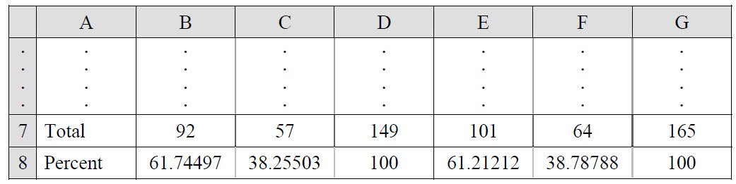
To see an example of this, suppose we wish to work out what percentage of each year’s sales were home and export; for example the Home percentage in 2003 would be 92×100/149 = 61.7%. Suppose we wish to calculate these percentages in row 8. To avoid having to type the same formula repeatedly, we can enter it once in cell B8 and then copy to cells C8:D8. The formula we use in cell B8 would be:
= B7*100/$D7 [= B7*100/$D$7 would produce the same effect]
Can we copy this same formula into cells E8:G8 to give the 2004 percentages? If not, what formula do we need in cell E8, which can then be copied to cells F8:G8?
Enter the correct formulae into cells B8 and E8, then copy and paste to complete row 8 as shown below:
Inserting Rows and Columns and Formatting Cells
As a final exercise, suppose we wish to calculate the quarterly percentage breakdown in total annual sales for each year. We could perform these calculations to the right of the data, in columns H and I. However, it would be better to put the 2003 percentages beside the 2003 data (i.e. between columns D and E) and the 2004 percentages after column G.
We need, therefore, to insert a new blank column after column D. To do this first position the cursor in the column immediately to the right of where the new column will be, and then click on Insert on the top menu bar, and choose Columns. A blank column will appear to the left of the cursor, and the columns to the right will be re-labelled. Rows can be inserted by a similar procedure.
Insert the blank column, which will now be column E, and calculate the percentage quarterly breakdown by entering and copying the appropriate formula. Notice that the formulae in both columns are essentially the same so if the correct formula is entered in cell E3, it can be copied to E4:E7 and I3:I7.
Finally, type in the heading “Percent” in cell A8, and copy it to cells E2 and I2.
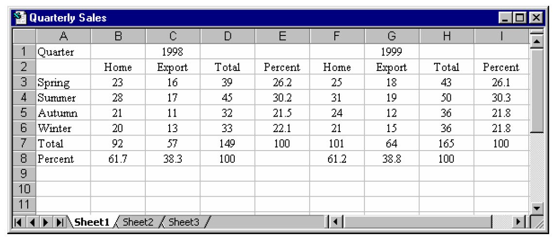
You will see that the percentage figures that you have calculated are given (by default) to 5 decimal places. In reality, this is unnecessary accuracy, and probably 1 decimal place is more than adequate. The contents of any cell can be displayed in a wide variety of ways to suit the purpose of the spreadsheet.
The format of cells is adjusted by selecting Format from the top menu bar, and choosing Cells. This allows you to change features such as alignment (left, right or centred), font and decimal places. More directly, you can set the alignment within any cell using the usual alignment buttons and increase/decrease the number of decimal places by clicking on the following buttons.
If you centre all the cells (apart from column A), and reduce the percentage figures to 1 decimal place, your spreadsheet should now look like that as shown in below screenshot.
Standard Functions
Suppose we need to enter a formula that calculates the total of 10 values entered in cells A1:A10. It would be very tedious to have to type in the following formula:
= A1 + A2 + A3 + A4 + A5 + A6 + A7 + A8 + A9 + A10
Fortunately, there is a shortcut. We can use a standard function for the sum of a range of cells. In the above case we could abbreviate the formula to = SUM(A1:A10)
The cells we wish to sum do not have to be in a single row or column; they could cover a number of adjacent rows and columns. For example, the total 2003 sales in cell D7 of Figure 2 could be written as = SUM(B3:C6)
Similarly, a number of distinct ranges could be included within the SUM function. For example, a formula for the overall sales for the two years could be written as = SUM(B3:C6, E3:F6)
SUM is just one of over two hundred standard functions, the majority of which you will probably have no need to use. The more commonly used functions are:
- SUM Sum of a range of cells
- MAX Maximum of a range of cells
- MIN Minimum of a range of cells
- SQRT Square root of a cell or value
- AVERAGE Average (arithmetic mean) of a range of cells
- STDEV Standard deviation of a range of cells
- MEDIAN Median of a range of cells
All functions that you will use require 1 or more arguments in brackets following the function name. These arguments almost always specify the cell or range of cells to which the calculation applies. If you know what arguments a particular function requires, you can simply type in the function name and its arguments as we did with the SUM function above.
A simpler way, however, is to use the Formulas menu and select Insert Function as shown below.
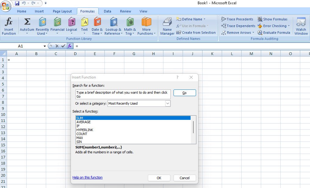
This brings up the Paste Function dialogue window from which you select the required function from the relevant category, for instance the basic mathematical functions are in the Math & Trig category, whereas the basic statistical functions (such as average and standard deviation) are in the Statistical category.
This then opens a dialogue box for the selected function which prompts you for the required arguments. The dialogue box for the SUM function is shown in Figure 6. An alternative to selecting function from the Insert menu is to click the function button .

- How To Fix the Crowdstrike/BSOD Issue in Microsoft Windows
- MICROSOFT is Down Worldwide – Read Full Story
- Windows Showing Blue Screen Of Death Error? Here’s How You Can Fix It
- A Guide to SQL Operations: Selecting, Inserting, Updating, Deleting, Grouping, Ordering, Joining, and Using UNION
- Top 10 Most Common Software Vulnerabilities
- Essential Log Types for Effective SIEM Deployment
- How to Fix the VMware Workstation Error: “Unable to open kernel device ‘.\VMCIDev\VMX'”
- Top 3 Process Monitoring Tools for Malware Analysis
- CVE-2024-6387 – Critical OpenSSH Unauthenticated RCE Flaw ‘regreSSHion’ Exposes Millions of Linux Systems
- 22 Most Widely Used Testing Tools